Problem Overview

This example introduces how to use the NastranIO class to read mesh information defined using Nastran bulk data format (BDF).

This example requires that MAST is compiled with the option ENABLE_NASTRANIO=ON and requires a Python interpreter with the pyNastran package be detectable by the MAST CMake build process on your system.

The mesh data that is read from the BDF input includes nodes, elements, subdomains for assigning properties, and node boundary domains for assigning boundary conditions.

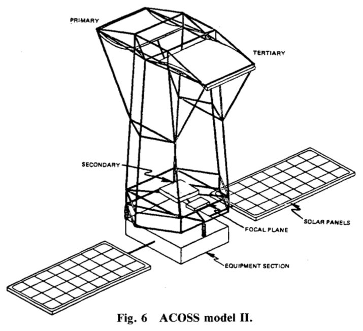
The geometry used in this example is a modified version of the of ACOSS-II (Active Control of Space Structures - Model 2) described in references [1] and [2], which has a compact BDF input suitable for use as a tutorial example. The ACOSS-II model has historical relevance as a demo case for optimal control of flexible structures and structural optimization with frequency constraints throughout the 1980's.

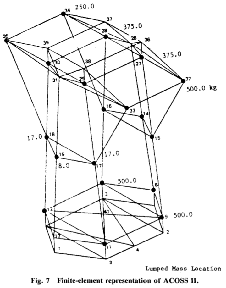
The mesh used in the example is taken from the ASTROS applications manual [3] and differs slightly from that in [2]. The basic geometry of the model is shown below:

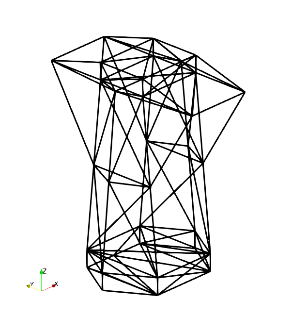
ACOSS-II (Active Control of Space Structures - Model 2)

(a) ACOSS-II configuration (from [2])	(b) ACOSS-II FEM representation (from [2])	(c) ACOSS-II MAST finite element model

We assume that the structure is modeled with beam elements and is made of a graphite epoxy material having Young's modulus 18.5x10 psi and mass density of 0.55 lb/in^3. We also assume currently that all elements have square cross section with dimensions 3.16 in by 3.16 in.

In the source listing below, we utilize components from the MAST library to setup a modal analysis of the modified ACOSS-II structure and calculate the first 10 vibration frequencies (eigenvalues) and mode shapes (eigenvectors). The structural mesh is read into libMesh/MAST using the NastranIO class.

The Nastran BDF mesh is located in the MAST source at: examples/structural/example_7/example_7_acoss_mesh.bdf.

To run this example with a direct solver (when linear solves are required inside the eigenvalue solver) use: mpirun -np #procs structural_example_7 -ksp_type preonly -pc_type lu.

TODO: Update this example to use actual truss elements with non-rectangular cross-section.

References:

Henderson, T.C., "Active Control of Space Structures (ACOSS) model 2," Draper Laboratory, Inc., Cambridge, MA., Technical Report C-5437.
Grandhi, R.V. and Venkayya, V.B., "Structural Optimization with Frequency Constraints," AIAA Journal, Vol. 26, No. 7, 1988., pp. 858-866.
Johnson, E.H. and Neill, D.J., "Automated Structural Optimization System (ASTROS) - Volume III Applications Manual," AFWAL-TR-88-3028.

# Documented Source Listing

Initialize libMesh library.

libMesh::LibMeshInit init(argc, argv);

Create Mesh object on default MPI communicator. – note that currently, NastranIO only works with ReplicatedMesh.

libMesh::ReplicatedMesh mesh(init.comm());

Create a NastranIO object and read in the mesh from the specified .bdf. Print out some diagnostic info for the mesh/boundary to see what was read in.

MAST::NastranIO nastran_io(mesh);
nastran_io.read("./example_7_acoss_mesh.bdf");
nastran_io.print_pid_to_subdomain_id_map();
mesh.print_info();
mesh.boundary_info->print_info();

Create EquationSystems object (a container for multiple systems of equations that are defined on a given mesh) and add a nonlinear system named "structural" to it. Set the eigen-problem type for the system so MAST knows we are eventually going to execute that solver. Also create a finite element type for the new system. Here we will use 1st order Lagrange-type elements and attach it to an initialization object, which provides the state variable setup for the equations corresponding to structural analysis.

libMesh::EquationSystems equation_systems(mesh);
auto& system = equation_systems.add_system<MAST::NonlinearSystem>("structural");
system.set_eigenproblem_type(libMesh::GHEP);
libMesh::FEType fetype(libMesh::FIRST, libMesh::LAGRANGE);
MAST::StructuralSystemInitialization structural_system(system, system.name(), fetype);

Initialize a new discipline, which we will utilize to attach boundary conditions.

MAST::PhysicsDisciplineBase discipline(equation_systems);

Create and add boundary conditions to the structural system. We use a Dirichlet BC to fix all of the nodes in SPC ID 1 in the .bdf file, which have been placed in a libMesh/MAST node boundary condition set with id of 1. Note that boundary condition application is not taken directly from the BDF definition, but simply the identification of which nodes are placed in the libMesh/MAST node boundary set. We specify which degrees-of-freedom for these nodes with DirichletBoundaryCondition.init(<boundary_id>, <variables>).

MAST::DirichletBoundaryCondition dirichlet_bc;
dirichlet_bc.init(1, structural_system.vars());   // Fix all variables in the system for
discipline.add_dirichlet_bc(1, dirichlet_bc);     // all the nodes in SPC ID 1.
discipline.init_system_dirichlet_bc(system);

Initialize the equation systems.

equation_systems.init();

equation_systems.print_info();

Initialize the eigen-problem and eigenvalue solver. Specify the number of eigenvalues that we want to compute.

system.eigen_solver->set_position_of_spectrum(libMesh::LARGEST_MAGNITUDE);
system.set_exchange_A_and_B(true);
system.set_n_requested_eigenvalues(10);

Create parameters.

MAST::Parameter thickness_y("thy", 3.16); // in
MAST::Parameter thickness_z("thz", 3.16); // in
MAST::Parameter E("E", 18.5e6); // lbf/in^2
MAST::Parameter nu("nu", 0.3); // no unit
MAST::Parameter rho("rho", 0.000142); // lbf*s^2/in^4 (0.055 lb/in^3 * 0.00259)
MAST::Parameter kappa_yy("kappa_yy", 5./6.); // shear coefficient yy
MAST::Parameter kappa_zz("kappa_zz", 5./6.); // shear coefficient zz
MAST::Parameter zero("zero", 0.0);

Create ConstantFieldFunctions used to spread parameters throughout the model.

MAST::ConstantFieldFunction thy_f("hy", thickness_y);
MAST::ConstantFieldFunction thz_f("hz", thickness_z);
MAST::ConstantFieldFunction E_f("E", E);
MAST::ConstantFieldFunction nu_f("nu", nu);
MAST::ConstantFieldFunction rho_f("rho", rho);
MAST::ConstantFieldFunction hyoff_f("hy_off", zero);
MAST::ConstantFieldFunction hzoff_f("hz_off", zero);
MAST::ConstantFieldFunction kappa_yy_f("Kappayy", kappa_yy);
MAST::ConstantFieldFunction kappa_zz_f("Kappazz", kappa_zz);

Create the material property card ("card" is NASTRAN lingo) and add the relevant field functions to it. An isotropic material in dynamics needs elastic modulus (E), Poisson ratio (nu), and density (rho) to describe its behavior.

MAST::IsotropicMaterialPropertyCard material;
material.add(E_f);
material.add(nu_f);
material.add(rho_f);

Create the section property card. Attach all the required field functions to it. A 1D structural beam-type element with square cross-section requires two thickness dimensions and two offset dimensions. Here we assume the offsets are zero, which aligns the bending stiffness along the center axis of the element.

MAST::Solid1DSectionElementPropertyCard section;
section.add(thy_f);
section.add(thz_f);
section.add(hyoff_f);
section.add(hzoff_f);
section.add(kappa_yy_f);
section.add(kappa_zz_f);

Specify a section orientation point and add it to the section. – Currently this orientation is arbitrary and we assume all beam sections are oriented in the same direction.

RealVectorX orientation = RealVectorX::Zero(3);
orientation(0) = 0.3583339;
orientation(1) = 0.8641283;
orientation(2) = 0.3583339;
section.y_vector() = orientation;

Attach the material to the section property, initialize the section, and then assign it to the subdomain in the mesh that it applies to. We note that we can reference the map between Nastran property IDs and libMesh/MAST subdomain IDs identify specific subdomains.

section.set_material(material);
section.init();
discipline.set_property_for_subdomain(1, section);

Create the structural modal assembly/element operations objects and initialize the condensed DOFs.

MAST::EigenproblemAssembly assembly;
MAST::StructuralModalEigenproblemAssemblyElemOperations elem_ops;
assembly.set_discipline_and_system(discipline, structural_system);
elem_ops.set_discipline_and_system(discipline, structural_system);
system.initialize_condensed_dofs(discipline);

Solve eigenvalue problem.

system.eigenproblem_solve(elem_ops, assembly);

assembly.clear_discipline_and_system();

Post-process the eigenvalue results. Get number of converged eigen pairs and variables to hold them.

unsigned int nconv_pairs = std::min(system.get_n_converged_eigenvalues(),

system.get_n_requested_eigenvalues());

Pre-allocate storage for calculations using the eigenvalues as well as storage for the eigenvector solution.

Real re = 0.0;
Real im = 0.0;
Real omega = 0.0;
Real freq = 0.0;
std::vector<libMesh::Real> solution;
equation_systems.build_solution_vector(solution);

Setup table for eigenvalue/frequency console output.

fort::table eigenval_out;
eigenval_out << fort::header << "Mode No." << "Eigenvalue"
             << "Frequency (rad/s)" << "Frequency (Hz)" << fort::endr;

Setup output files to save frequency data and mode shapes.

std::ofstream freq_csv;
if (init.comm().rank() == 0) {
    freq_csv.open("freq_data.csv");
    freq_csv << "Mode Number, Real Eigenvalue, Angular Frequency (rad/s), Frequency (Hz)" << std::endl;
    freq_csv << std::scientific;
}

Exodus output file for mode shapes.

libMesh::ExodusII_IO exodus_writer(mesh);

Loop over and process data for each vibration mode.

for (unsigned int i = 0; i < nconv_pairs; i++) {

Get eigenvalue/eigenvector pair.

system.get_eigenpair(i, re, im, *system.solution);

Get eigenvector on Rank 0 solution.

system.solution->localize_to_one(solution);

Calculate frequency for current eigenvalue.

omega = sqrt(re);

freq = omega/2.0/M_PI;

Add data to console output table.

eigenval_out << std::to_string(i + 1) << std::to_string(re)

<< std::to_string(omega) << std::to_string(freq) << fort::endr;

Write frequency results to text file (only from rank 0 processor).

if (init.comm().rank() == 0) {
    freq_csv << i + 1 << ", " << re << ", " << omega << ", " << freq << std::endl;
}

Write currently active eigenvalue into Exodus file.

exodus_writer.write_timestep("mode_shapes.exo", equation_systems, i + 1, i);

}

Output eigenvalue/frequency table to console.

libMesh::out << eigenval_out.to_string() << std::endl;

Results

Successful execution of the example should produce both console output and files. Tabular output showing eigenvalues, angular frequencies (in rad/s), and frequencies (in Hz) correpsonding to the first 10 vibration modes should be output to the console. This output should be similar to the following values:

Mode No.	Eigenvalue	Frequency (rad/s)	Frequency (Hz)
1	520.408008	22.812453	3.630715
2	2263.881979	47.580269	7.572635
3	3475.185118	58.950701	9.382295
4	7543.959254	86.855968	13.823557
5	7824.872647	88.458310	14.078577
6	11756.804335	108.428798	17.256979
7	13055.444785	114.260425	18.185111
8	53884.048267	232.129378	36.944538
9	63204.791232	251.405631	40.012449
10	86174.214772	293.554449	46.720642

In addition, two output files should be produced. freq_data.csv contains console output in .csv format that is suitable for external post-processing. mode_shapes.exo contains the mode shape data in the Exodus-ii format, which can be opened for visualization in Paraview.

The mode shapes corresponding to the first 9 vibration modes are shown below:

Vibration Mode Shapes

Mode 1	Mode 2	Mode 3

Mode 4	Mode 5	Mode 6

Mode 7	Mode 8	Mode 9